R packages

We will use the R packages leaflet to produce the map, ggmap to obtain the coordinates of the locations, and geosphere to obtain the great circle arcs between the locations. Then we will use packages savewidget and htmlwidgets to get a static png version of the map. Data we will use is in the epimaps package.

library(leaflet)
library(ggmap)
library(geosphere)
library(htmlwidgets)
library(webshot)
library(epimaps)

Data

To make this plot we need two data.frames.

The first data.frame is called loc_lat_long and it contains the following variables:

• locs: code of locations
• lat: latitude
• long: longitude

The second data.frame is origin_end_count and it contains the variables

• origin: code of origin locations
• end: code of destination locations
• count: number people flying between the locations

In this example we will use the populations flows to Mexico from other countries in year 2009 that are in the dataset Mex_travel_2009 from the epimaps package. We will use the function geocode from the ggmap package to obtain the coordinates of the countries.

# Countries of origin
locations<-as.vector(Mex_travel_2009[[2]]$country)
# Get coordinates of countries
long_lat <- geocode(locations)
# Create data.frame loc_lat_long
loc_lat_long <- data.frame(locs = locations, lat=long_lat[,2], long=long_lat[,1])


# Number people travelling to Mexico from other countries
number_people <- Mex_travel_2009[[1]]$MEX
# Create data.frame origin_end_count
origin_end_count <- data.frame(origin = locations, end = rep("Mexico", length(locations)))
origin_end_count$count <- number_people

Calculate great circle arcs for each connection

We use the function gcIntermediate from the geosphere package to get the intermediate points on great circle arcs between locations, and store them as a SpatialLinesDataFrame that we will pass to the leaflet function.

listlines<-list()
for (i in 1:nrow(origin_end_count)) {

  # latitude and longitude of origin and end locations
  origin <- loc_lat_long[loc_lat_long$locs == as.vector(origin_end_count[i,]$origin),]
  end <- loc_lat_long[loc_lat_long$locs == as.vector(origin_end_count[i,]$end),]

  # Get intermediate points on a great circle between the two locations
  # We set  sp=TRUE to retrieve a SpatialLines object
  connection <- gcIntermediate(c(origin[1,]$long, origin[1,]$lat), c(end[1,]$long, end[1,]$lat),
                          n = 100, addStartEnd = TRUE, sp = TRUE)
  listlines[[i]] <- Lines(connection@lines[[1]]@Lines, ID = i)
  
}

sl <- SpatialLines(listlines)
sldf <- SpatialLinesDataFrame(sl, data.frame(count = origin_end_count$count))

Plot

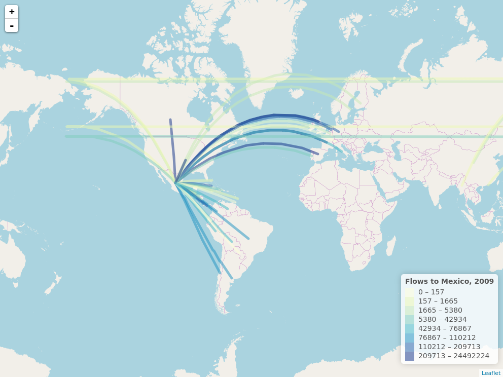
Now, we create a leaflet map with the connections. Lines are coloured according to the flow volume. As the mouse passes over the lines, lines highlight and information about connections is shown.

pal <- colorQuantile(palette = "YlGnBu", domain = sldf$count, n=8)

labels <- sprintf("%s to %s: %s", origin_end_count$origin, origin_end_count$end, origin_end_count$count) %>%
  lapply(htmltools::HTML)
 
m <- leaflet(data = sldf) %>%
  setView(lng = -50, lat = 20, zoom = 2) %>%
  addTiles(urlTemplate = "http://{s}.tile.openstreetmap.org/{z}/{x}/{y}.png") %>%
  addPolylines(data = sldf, color =  ~pal(count),
               highlightOptions = highlightOptions(color = "black", weight = 2), label = labels) %>% 
  addLegend("bottomright", pal = pal, values = ~count, title = "Flows to Mexico, 2009",
            labFormat = function(type, cuts, p) {
              n = length(cuts)
              paste0(cuts[-n], " &ndash; ", cuts[-1])
              })
  
m

Save leaflet map as a static png file

Finally, to save the leaflet map as png we will first save it as an HTML file with the function savewidget from the htmlwidgets package, and then capture a static png version of the HTML using the function webshot of the package webshot.

saveWidget(m, file = "flowsmap.html", selfcontained = FALSE)
webshot("flowsmap.html", file = "flowsmap.png", cliprect = "viewport")